101: Weather Radar (Velocity)

Radar Radial Velocity


Doppler and Pulse-Pair Processing

In 1842, Austrian physicist Christian Doppler proposed the theory that would eventually be named after him: the Doppler effect. A Doppler shift is the change in frequency of some periodic signal due to the emitting object's velocity relative to the observer. Sound, which is made up of pressure waves (a type of periodic pulse) is the most commonly experienced source of Doppler shifts. Whenever a moving object, such as a car or airplane, is approaching the observer, the pitch of the sound will seem higher to the observer than to one moving at the same speed of the object (figure 1). As the object passes the observer, the pitch will seem to lower. At all times the object is emitting the same frequency sound, but to an observer it is approaching, the sound waves will seem compressed, resulting in a higher frequency sound. The reverse is also true when the object is moving away and the observer receives the sound waves at a lower frequency. The original purpose of defining the Doppler effect was to explain the shift in the color of distant stars and galaxies (figure 2). In this case, the lengthening of the light waves causes the frequency to appear longer to an observer on Earth, resulting in a shift towards the red end of the visible spectrum. In astronomy, this color change is used to gauge the rate of the universe's expansion and is expressed in a value known as redshift. For all uses of the Doppler effect, it is imperative to remember that it only indicates the velocity towards or away from the observer. If an object were to be moving at a right angle to the observer's line of sight, there would be no shift.

Figure 1: Sound waves emitted by a moving vehicle get compressed in front of it and stretched behind it.

Figure 2: To an observer, the wavelength of light waves emitted by stars moving away from an observer appears to lengthen (shift towards the red end of the visible spectrum), while a star moving towards the observer appears to be bluer than it actually is.

In the case of weather radar, things get a little more complicated. Suppose a radar beam is sampling a target in a tornado moving toward the radar at about 100 kt and assume the frequency of the light leaving the beam is about 2850 MHz. Since the target is moving towards the radar, the frequency of the backscattered beam should be greater than what was emitted. In this case, the backscatter would have a frequency of of about 2850.00001 MHz. A shift of 0.00001 MHz is far beyond the ability of the radar unit to measure accurately, thus another technique must be applied.

In order measure the radial velocity of a radar target, the radar does not look for a shift in the frequency of the backscatter, but the difference in the phase between two different pulses. If the light being received by the radar unit is thought of as a wave, then its sine wave shape can be graphed. Consider a target that is neither moving towards or away from the radar. The shape of the waves being received by two consecutive pulses would be the same (figure 3). However, if the target is moving away from the radar, the second pulse will have to travel slightly further to sample it, thus the wave shape would be shifted a little relative to the shape of the first pulse's wave when it arrives back at the radar unit; this difference is measured in degrees (figure 4). Higher velocity targets will cause a greater shift in the shape. The maximum difference occurs when the two waves are 180 degrees shifted relative to each other (figure 5). A problem arises when a target causes the shift to go beyond 180 degrees: the radar gets confused as to how the waves have changed. For instance, if a target were to cause a shift of 200 degrees, the radar would interpret this as -160 degrees because sin(200 degrees) and sin(-160 degrees) have the same wave shape (figure 6). Therefore, the radar assumes all phase shifts are between -180 and 180 degrees, thus a target moving such that it causes a shift slightly more than 180 degrees will actually appear to be moving at nearly the same speed, but in the opposite direction. This issue is known as aliasing, and the maximum speed that a radar can record without being aliased is known as the maximum unambiguous velocity. For the WSR-88D the greatest velocity possible is 64 kt, although some VCPs are even lower.

Figure 3: A target that is not moving will cause two consecutive pulses to have an identical shape.

Figure 4: A target moving away will cause consecutive waves to be offset (shifted).

Figure 5: A target moving away at the fastest measurable speed will cause waves to be shifted to appear to be a mirrored version of each other.

Figure 6: Just past the maximum measurable speed, the second wave will be indistinguishable from a wave moving nearly the same speed in the opposite direction. In this case, a shift of 200 degrees looks the same as a shift of -160 degrees.

In order for higher speeds to be measured, the time between pulses must decrease, since this will require higher speeds in order to shift the wave 180 degrees between the two pulses. However, shortening the interval between pulses causes the maximum range of the radar to decrease due to range folding. The required compromise between the two factors is known as the Doppler dilemma. Luckily, modern radar unit programming allows the beam to be dealiased by looking for continuity between gates (figure 7). This is built in to level III velocity products and some end-user radar display programs can dealias level II data. Despite this, an observer must look out for any a errors as dealiasing is not 100% effective.

Figure 7: On the left is the level III dealiased version of the level II data on the right. Notice how the bright green (fast inbound) gates near the center have been corrected to be bright red (fast outbound). In this case, a tornado was occurring an was producing radial velocities greater than about 53 kt, the maximum speed the radar could measure in this mode (VCP 212).

Finally, velocity data is highly prone to range folding, and unlike reflectivity data, cannot be unfolded. Thus, areas that are experiencing range folding are usually present in velocity images and are marked as such, usually with a dark purple color. These "un-unfoldable" areas are also present in some of the other base products and can result considerable complications when analyzing the radar data.



Spectrum Width

Despite being one of the three original base products produced by the WSR-88D, spectrum width is notable in that it has received little attention from both research and operational meteorologists. Essentially, spectrum width is the diversity of radial velocities sampled in each radar gate and is expressed as a standard deviation. In cases such as light drizzle, where droplets are roughly the same size and shape, spectrum width will be low since all the sampled targets have similar aerodynamic properties and thus are moving uniformly with the wind. On the other hand, around an updraft of a strong thunderstorm spectrum width will be very high, since those gates will likely contain water droplets, large rain drops, ice crystals, and snow; all of which have very different aerodynamic properties and thus will move at different speeds and directions.

While not widely used, spectrum width has some significant potential uses in severe weather situations. One key use of the product is to identify boundaries, even if they are obscured by precipitation. Boundaries such as gust fronts can provide significant rotation to a thunderstorm's updraft, which can lead to severe hail and tornadoes. While gust fronts show up on reflectivity, they may be impossible to distinguish if they are embedded in precipitation. However, the chaotic nature of the targets moving along with the boundary will show up as a line of high spectrum width. This product has also shown some promise in identifying tornadoes, even if they are rain shadowed. After all, tornado debris made of a wide range of shapes and sizes, leading to very different velocities.



Level II Base Radial Velocity

Like reflectivity, the level II data of velocity can be used to create 3-D displays. Cross sections can help the user identify vertical signature of a tornado by identifying areas of strong inbound velocity directly adjacent to areas of strong outbound velocity (figures 11 through 14). Mesocyclones, the rotating core of supercell thunderstorm, can also be detected as in the same manner of tornadoes, but at a higher elevations, generally weaker velocities, and covering a larger area (figure 12). Velocity cross sections can also identify rear inflow jets, which are a feature found in many squall lines that can signal the descent of destructive straight-line winds to the surface (figure 16). These features can also be detected using isosurfaces and radar volumes by choosing the right parameters, but these will often be noisy and difficult to interpret (figures 13 and 14).

Figure 8: The idealized structure of a supercell thunderstorm with the locations of the tornado and mesocyclone labeled.

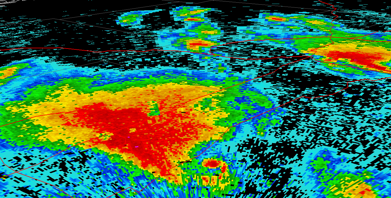Figure 9: The images in this post are from a severe weather outbreak in the Dallas/Ft. Worth area on April 3, 2012. This scan from 1:27 CDT (1827 UTC) was also used in figure 8. Looking to the northeast, the supercell in the foreground included a tornado inflicting EF-2 damage near Kennedale; the circle of reflectivity near the bottom of the image is from the debris the tornado was lofting into the air. This tornado caused roughly 200 million dollars in damage and the supercell further to the east had also spawned a EF-2 tornado that caused about 400 million dollars in damage.

Figure 10: A 45 dBZ isosurface from the same scan; the Kennedale tornado can be vaguely identified as a semi-isolated column in the center of the image.

Figure 11: A 0.5 degree velocity image from the same time as figure 8, but from a different angle.

Figure 12: A velocity cross section revealing the vertical profile of the rotation due to the tornado (lower down) and the wider mesocyclone (upper portion). The image is contaminated by aliasing (the erroneous bright green gates on the right side of the lower circulation) over a considerable depth of the tornado's signature.

Figure 13: An isosurface of the -20 kt (20 kt inbound) radial velocity. The bright side of the column is the aliased outbound signature, while the duller green on the left side near the base of the column is the actual inbound velocity. Because the storm was moving away from the radar, the inbound velocities associated with this supercell were generally lower than the outbound velocities.

Figure 14: A volume scan does not help much in with velocity data, though the column of aliased velocities can be identified here.

Figure 15: The 0.5 degree spectrum width shows high values in the updraft area of the storm (the right side, near the bottom of the image) and associated with the tornado debris (immediately below and to the left of the main updraft area).

Figure 16: A little later in the day (3:33 CDT, 2033 UTC) a squall line moved through the area. The velocity cross section shows strong winds associated with the rear inflow jet (lower red area) being brought down towards the surface while the updraft flow (lower right to upper green area) was inbound. Notice the small amount of aliasing in the jet and in the upper right where strong upper-level winds are blowing the storm's anvil downwind.

Level III Products (and their product codes)

Level III Base Velocity (N0V, N1V, N2V, N3V, N0W, and many others)
These are simply flat, individual files of the lowest few tilts of base velocity. They are analogous to the level III base reflectivity products in that they have undergone some quality control and have been largely dealiased (figure 17). Unlike their reflectivity counterparts, however, they still retain areas of range folding.

Figure 17: The level III image of the radial velocity and reflectivity of the Kennedale tornado and its parent supercell.

Level III Base Spectrum Width (NSP, NSW)
Spectrum width comes in two different level III formats: NSP is a high resolution product (figure 18) that has a range of just 32 nautical miles (nm), while NSW is somewhat lower resolution with a range of 124 nm. Like the velocity products, these likely contain data that cannot be unfolded.

Figure 18: Level III spectrum width (the higher quality 32 nm version) from the same scan as was used in many of the previous images. Note that the color table used here is more typical of spectrum width images than the one used in figure 15.

Storm Relative Velocity (N0S, N1S, N2S, N3S)
Because storms are always moving with respect to the ground, internal rotation in the storms, such as tornadoes and mesocyclones, can be hard to identify. Storm relative velocity products attempt to fix this by using the storm track vectors (from the reflectivity products) to decide what the average speed and direction the storms being sampled are moving in. This motion is subtracted from the base velocity data to create a product that depicts the storms as if they were stationary (figure 19). This product should always be used in all severe weather events, except when attempting to locate downbursts of wind.

Figure 19: In the storm relative velocity product, the outbound velocity of the overall storm is subtracted from base radial velocity data to provide a clearer picture of the rotation associated with the Kennedale tornado.

VAD Wind Profile (VWP)
The wind profile product uses all tilts and the entire sweep of the radar to estimate the environmental wind speed and direction at 500 or 1000 ft increments based on the output from the Velocity Azimuth Display (VAD), which is rarely viewed by itself. The data is displayed as a graph of wind barbs (similar to the kind seen on weather maps) arranged in a column, along with columns of the wind profiles from up to the 10 preceding scans (figure 20). Each barb is color coded to indicate the level of confidence in the measurement. Since this product assumes that at each level the wind is moving in the same direction across the entire range of the radar, care must be taken if a sharp wind shift, such as a front, is present in the area as this could lead to very high error.

Figure 20: The VWP graph from earlier in the day (times shown are in UTC and height is in thousands of feet) indicate the wind was from the southeast near the surface then shifted to a strong south-southwesterly wind aloft. Most of the wind barbs in these scans are green or yellow, indicating high or moderate confidence in the data, although a few low confidence red barbs are present.

Mesocyclone (NME, NMD)
The rotating cores of supercell thunderstorms are important to locate because they hint at the health and strength of the storm, as well as being directly associated with the formation of tornadoes. The radar's Mesocyclone Detection Algorithm (MDA) detects mesocyclones in much the same way the storm tracking product detects thunderstorm cells: by finding the centroid. However, unlike the storm track, the MDA looks for a centroid of rotation in the storm and attempts to track it from scan to scan. If it finds a consistent signature, it labels the location with a mesocyclone symbol (figure 21). On many radar display products, this is indicated by a circle or two curved arrows forming a circle. If the mesocyclone does not extend to the base of the cloud, a broken circle will be used instead to indicate an elevated mesocyclone. Finally, each symbol is color coded to indicate its intensity. In areas where topographical feature create chaotic wind currents, the MDA does have a tendency to "detect" a mesocyclone even if none exists.

Figure 21: At 3:37 CDT (2037 UTC) the radar captured a supercell that produced EF-3 damage to the town of Forney, east of Dallas. Here, the mesocyclone product has identified the rotating core of the storm and its details are displayed in the overlaid box and in the storm attributes table. Note that the mesocyclone symbol marks the center of rotation, the full extent of the structure is much larger than the icon.

Tornadic Vortex Signature (NTV)
The Tornado Detection Algorithm (TDA) works in a similar manner to the MDA, but looks for the much smaller tornadic vortex signature (TVS) of a tornado (figure 22). Although similar to the mesocyclone product, the TDA is computed entirely independent of the MDA. Therefore if a TVS is located within (or very close to) a mesocyclone signature, greater confidence can be placed in the likelihood that a tornado does in fact exist (figure 23). On radar display products, TVSs are typically indicated by an upside-down triangle with a number indicating its intensity. If the tornado is elevated (not yet reaching the ground) an ETVS is indicated with a hollow triangle. Like the MDA, the TDA is quite prone to error, especially where topography is affecting air currents. Spotter reports are the only way to conclusively determine if a tornado actually is occurring.

Figure 22: The TVS associated with the Forney tornado was also captured by the radar. Its details are also displayed in the overlay and storm attributes table. At this range, each of the gates is far larger than the actual tornado (which had a maximum width of about 150 yards) so the precise location of the TVS icon should be considered an estimate.

Figure 23: Here the mesocyclone and TVS are both displayed. The fact that they overlay so well, and are associated with the hook echo in the reflectivity product indicates high confidence that a tornado is actually occurring.