101: Weather Radar (Polarimetry)

Much of the science behind dual-polarimetric radar concepts is rather complicated, so only basics will be covered here. For a more in-depth explanation see the National Weather Service's manual here and an extended one from their training course here.



Dual-Polarimetric Radar


Polarimetry

Scientifically speaking, light is nothing more than a type of electromagnetic energy. When conceptualized as a wave, electromagnetic energy is comprised of two oscillations: an electric wave and a magnetic wave (figure 1). These two components are oriented at right angles to each other and are self-propagating. This means that the electric wave induces the magnetic wave, which then induces the electric wave, and so on. These two waves have a specific orientation when emitted. In the case of television broadcasts, the waves are oriented with the electric field component horizontal to the ground, therefore they are considered to be horizontally polarized. Traditionally, weather radar has also been horizontally polarized, which is useful since most rain drops flatten out as they descend. However, rain is not the only target radars pick up on, thus having multiple polarities yields more information about what the radar is seeing.

Figure 1: The basic representation of an electromagnetic wave. The E axis is the electric wave, the B axis is the magnetic wave, and z is the direction of propagation. The distance indicated by the brackets is one wavelength. In this case, the beam would be considered vertically polarized.

Although the concept of radar with multiple polarization dates back to WWII, the first radars to actually implement it did not come about until the 1970s. However, this was limited to a few research radars, since the computing power required to process various polarity signals simultaneously and in real time did not exist on a large scale. As computing power matured, the concept of a dual-polarity ("dual-pol") radar network was considered. The remaining limiting factor was the cost of the hardware itself. To create a dual-pol network, radars would have to include equipment that switched the polarity of the beam from horizontal to vertical rapidly. Such a configuration would be far too expensive to implement. Furthermore, requiring the beam to constantly switch polarity would greatly increase the time the radar would need to complete a volume scan. The solution was to take existing radar hardware and adjust it to emit a beam at a 45 degree angle to the vertical. When this beam was backscattered back to unit, the radar's computer would separate the horizontal and vertical components of the signal and compare them as if two separate signals had been emitted. With the software and hardware now available, the National Weather Service approved a conversion of all existing WSR-88D units into dual-pol radars in 2003 and by the end of 2013 the entire NEXRAD network had been updated (figure 2).

Figure 2: The Lubbock, TX, radar (KLBB) being upgraded for dual-pol capability.

Dual-pol radar allows for the comparison of the strength of the horizontal and vertical components of the beam (figure 3). This does not mean the radar is able to directly detect the actual horizontal and vertical dimensions of the targets its sampling, only the general shape of the targets. This can be compared to observing a large cluster of buildings from far away. It is impossible to know how tall or wide the buildings are, but it is possible to compare their height to their width. With this knowledge, one can make some inferences about the nature of those buildings, even if their actual size is unknown. For example, observing a large cluster of buildings that were many times taller than they were wide might indicate to the observer that the buildings were part of the downtown area of a major city. On the other hand, a large number of building that were much wider than they were tall could mean they were part of an industrial district full of warehouses. Finally, a cluster of buildings whose width was generally similar to their height would likely indicate a suburban neighborhood with lots of one or two story houses. Dual-pol radar works in much the same way, however it expresses its information in the form of three different base products: differential reflectivity, correlation coefficient, and specific differential phase. The products are packaged along with the original three base products (reflectivity, velocity, and spectrum width) in the level II data stream of all dual-pol radar data.

Figure 3: Conceptual diagram of the two different polarities measured by dual-pol radar. The E indicates that the electric portion of the wave is being shown.

Differential Reflectivity

Commonly abbreviated as ZDR, differential reflectivity is the ratio of the power returned in the horizontal from that returned in the vertical (figure 4). Like traditional reflectivity, ZDR is expressed in dBZ (some sources label express it in units of dB), a logarithmic unit (i.e. ZDR=10*log(horizontal reflectivity/vertical reflectivity)).  Therefore, positive values indicate stronger returns in the horizontal, while negative values indicate predominately vertically polarized reflectivity. Thus, this product provides information on the shape of the targets and values typically fall between -2 and +6 dB.

Figure 4: Comparison of differently shaped targets and how they affect the ZDR value. The values of Z with subscripts H and V refer to the horizontal and vertical polarity of reflectivity, respectively.

Since large rain drops, typically associated with heavy convective showers, tend to flatten out as they fall due to drag, areas of heavy rain will typically have ZDR values of at least 3 (figure 5). On the other hand, large hail that has accreted from multiple smaller stones tend to take on more of an irregular shape. When these fall, they tend to orient themselves vertically due to wind, generally resulting in ZDR values between -1 and 0. Very light rain, snow, ice crystals, and small hail tends to yield a ZDR near zero due to their relatively spherical nature (figures 6 and 7). Tornado debris also tends to appear as near zero values, not because the particles of debris are spherical, but because they are of all different shapes (and often rotating rapidly) the net result is nearly equal returns in the horizontal and the negative (figure 6). Biological targets such as birds and insects generally produce very large positive ZDR values because their wings are typically oriented horizontally.

Figure 5: Drop size affects its shape and therefore its ZDR value as these images of drops captured on high speed camera during a laboratory experiment demonstrate.

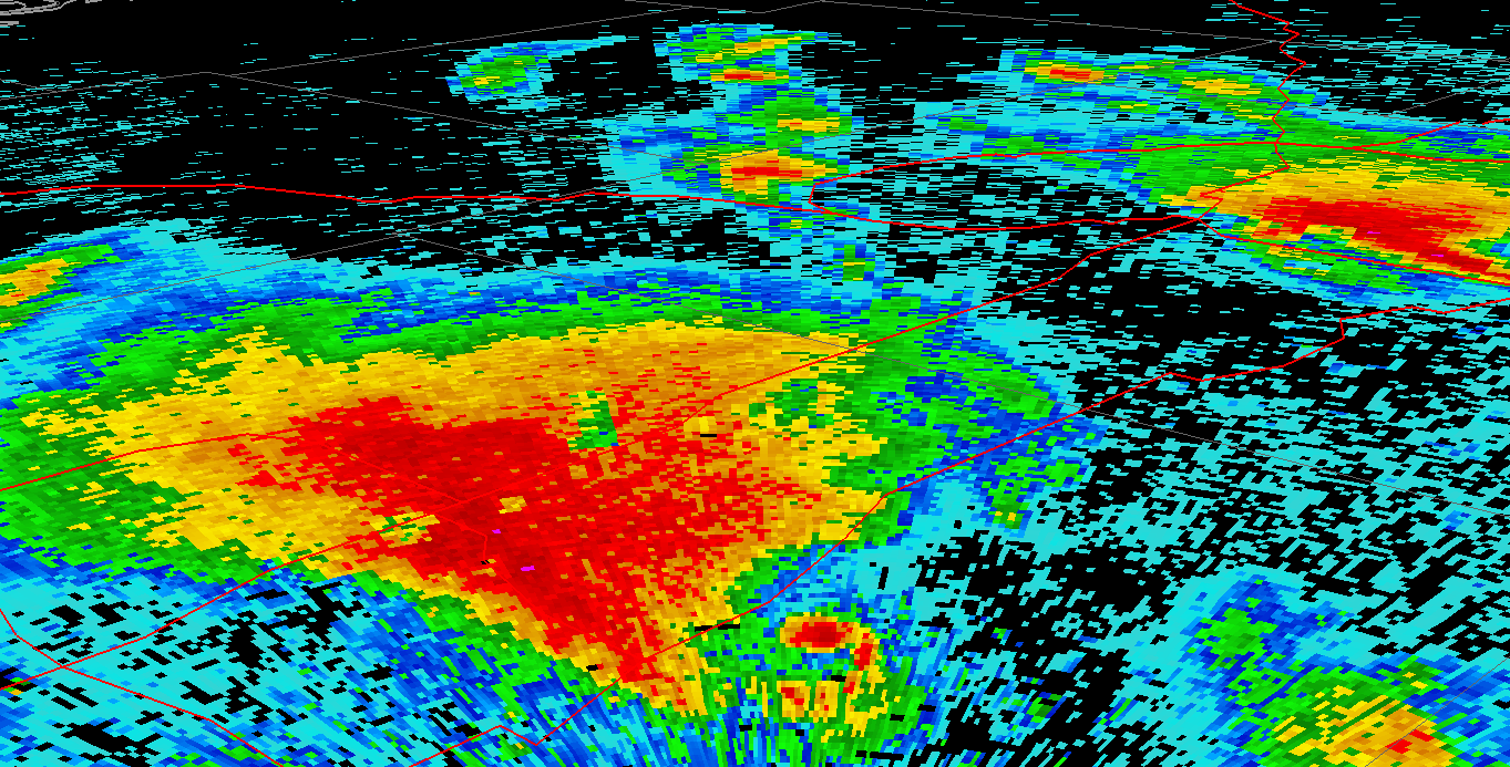
Figure 6: ZDR and reflectivity data of the supercell that produced the EF-5 Moore, OK, tornado on  May 20th, 2013. This scan is from 2003 UTC and two unique ZDR signatures, highlighted by the white boxes. In the southwest portion of the image is the debris ball produced by the tornado. The debris itself produced a very noisy signal, but overall the values tended to be around 0 dB. To the north, hail was occurring, which also resulted in ZDR values near 0 dB. Neither of these features are immediately obvious from the reflectivity image alone. The 0.9 degree tilt was used here instead of the 0.5 degree tilt due to the storm's close proximity to the radar (the tornado was about 15 nautical miles (nm) away from the radar (KTLX) at the time).

Figure 7: These two supercells formed during the same 2013 outbreak. The ZDR image uses a high tilt which, judging by the generally low values, intersected the storm above the melting layer. However, a few isolated areas of high values do occur. The cluster of high values near Purdy (about 40 nm south-southwest of the radar) represents the updraft core of the storm, which is lofting water drops above the freezing level before they have a chance to freeze. These are called ZDR columns and they are useful in identifying the core of severe storms.

Figure 8: This cross-section directed towards the northeast away from the radar intersected several storms. While noisy, most gates drop down to near 0 dB around 11,000 feet, the level of the white line, which indicates this is the top of the melting layer. A few spikes of higher values above the line are ZDR columns from various storms.

Correlation Coefficient

Often referred to simply as CC or the Greek letter rho, correlation coefficient compares the consistency between the returned power in the horizontal from that in the vertical. Therefore, little change in the orientation of targets from pulse to pulse results in high values, while inconsistent returns produce a low value. CC is expressed in unit-less values between 0 and 1, or as a percent between 0% and 100%. In general CC values between 0.97 and 1 are considered high, between 0.95 and 0.96 medium, 0.6-0.94 low, and 0-0.6 very low. Low and very low values are generally due to non-meteorological targets, medium values are often associated with a high diversity in hydrometeor (the general term for all types of precipitation) types and shapes, and high values are associated with uniform precipitation that does not consist of particles that change orientation significantly (figures 9 and 10).

Figure 9: The same frame used in figure 6 is used here to show the incredibly low CC values the tornado debris produced. The area of hail to the north, which was likely mixed with some rain, also produced relatively low values. Regardless of their reflectivity intensity, precipitation outside these areas tended to have high values due to their uniformity.

Figure 10: Looking at the reflectivity image, it appears that a small shower was occurring over Seattle, WA, just after midnight on New Year's day, 2016. However a look at the very noisy CC signal indicates otherwise. The night was perfectly clear and the "shower" was actually smoke from a large fireworks display happening at the Space Needle.

One key strength of CC is its ability to highlight the melting layer. As frozen precipitation falls below the freezing level it begins to melt. While melting, these hydrometeors consist of ice coated with a layer of liquid water, resulting in high reflectivity values. On a radar display of reflectivity, this zone will appear as a "bright band" of high values, since the beam gets higher with distance. From the freezing level to the level in which all the ice has melted (leaving only rain drops) there is a wide variety of shapes present that all have different aerodynamic properties and therefore fall in slightly different ways. As a result, this melting layer will have often have CC values less than 0.95, while above and below the layer values will be very close to 1 (figures 11 and 12).

Figure 11: This area of precipitation near the TX/LA border on January 6, 2016, shows the bright band in both CC (left) and reflectivity (right). The rings indicate the top and bottom of the melting layer. A high tilt was used to capture higher parts of the precipitation and to lessen the noise that often occurs closer to the ground.

Figure 12: A CC cross section along the leading edge of the main area of precipitation shows the lower values associated with the bright band, the center of which is indicated by the white line.

Specific Differential Phase

This product, also known as KDP, essentially applies the concept used in radial velocity measurements to the two component polarization returns and compares them. The basis of this product is a value known as differential propagation phase (sometimes simply called differential phase). To conceptualize this measurement, consider the wave shape concept introduced in the velocity post. Recall that differences between two pulses' waves, the phase shifts, were expressed in units of degrees. To obtain differential phase the phase shift to the vertical component is subtracted from the phase shift to the horizontal component. Differential phase is additive along each radial; that is, the value will change every time the beam passes through precipitation as it propagates outward without returning to any base value. For example, imagine there are two rain shafts the radar beam encounters along a radial: the first causes a differential phase of 11 degrees, and the second causes 14 degrees. The value along the radial would be 0 until the first shower, after which each gate would keep the value of 11 degrees until reaching the second shower. After the second shower the remaining gates in the radial would not have a value of 14 degrees, but 25 degrees (the total shift), since the value never reverted back to 0. This property gives radar images of differential phase a streaked appearance that makes interpretation difficult (figure 13).

Figure 13: The differential phase image of supercells, some of which were featured in figure 7, says very little about the storms except that the beam must have passed through some heavy, non-spherical targets, as indicated by the red and purple streaks.

To address the issue differential reflectivity produces, specific differential reflectivity (KDP) presents difference per kilometer. Thus KDP is displayed in values of degrees per kilometer. In the example used above, KDP would be 0 between the two showers since the value of differential phase was not changing along that portion of the radial. Essentially, KDP is the gradient of differential phase with distance; the more differential phase changes with distance, the greater the KDP value. This product has been found very useful for detecting heavy rain, as that produces high KDP values, while filtering out most spherical hydrometeors, since they behave similarly in both the horizontal and vertical (figure 14). Thus, in winter weather situations, KDP can help single out areas of liquid rain. Unfortunately, the archived level II data only offers differential phase; KDP is only available in NWS offices and as level III data.

Figure 14: The KDP image of the same storms as in figure 13 is much more meaningful and  highlights areas of heavy rain.

Level III Products (and their product codes)


Level III Differential Reflectivity (N0X, N1X, N2X, N3X, and others)
These are simply flat, individual files of the lowest few tilts of base ZDR with some quality control.


Level III Correlation Coefficient (N0C, N1C, N2C, N3C, and others)
These are simply flat, individual files of the lowest few tilts of base CC with some quality control.


Level III Specific Differential Phase (N0K, N1K, N2K, N3K, and others)
These are simply flat, individual files of the lowest few tilts of base KDP with some quality control. Note that this is specific differential phase, not differential phase (which is not offered as a level III product).

Melting Layer (N0M, N1M, N2M, N3M, and others)
The Melting Layer Detection Algorithm (MLDA) uses ZDR and CC to try to identify the bright band by assuming it is comprised of wet snow. In cases where there is not enough echoes to reliably establish the melting layer, the MLDA uses elevations provided by either the radar operator or the most recent computer weather model output. In radar programs that support the display of the melting layer, the data will appear as four overlaid rings; typically two bold rings in the middle and two dull or dashed rings on either side of the bold ones. Since the radar beam's altitude increases with range, the rings' radius acts as sort of a proxy for their height above ground. The inner bold ring represents the altitude that the center of the beam enters the melting layer while the second bold ring represents where the center of the beam exits the melting layer. Furthermore, the innermost ring (dull or dashed in appearance) corresponds to the height at which the top of the beam enters the melting layer, while the outermost ring (dull/dashed) represents where the bottom of the beam leaves the melting layer. Therefore, all mixed phase precipitation should fall somewhere between the inner and outermost rings.

The MLDA is not without its own issues, however. In cases of intense convective updrafts the melting layer will increase locally, which may or may not be captured by the MLDA. Furthermore, the radar assumes that once the precipitation has melted, it will not refreeze. In winter weather situations, such as the area just to the cold side of a warm front, a layer of cold air will exist near the surface. If this layer is deep and/or cold enough, precipitation will refreeze and sleet or ice crystals will occur at the surface. Since this will not be picked up by the MLDA, those using radar data should check to see if there is a sharp increase in ZDR or decrease in CC below the identified melting layer if a refreezing layer is suspected (figure 15). Finally, small zig-zag patterns often appear on the melting layer rings (figure 16). Since the MLDA is highly sensitive to the radar's tilt, the slight wobble that occurs as the radar settles after it changes its tilt during scanning will produce these small errors. The longer the radar takes to complete a scan, the more errors will occur. Therefore, in clear air modes, such as VCP 32, far more errors will be noticeable than in fast scans such as VCP 12.

Figure 15: An ice storm near Grand Rapids, MI, on December 22, 2013 illustrates a shortcoming of the MLDA. The CC image on the left indicates that the melting layer, marked by the white rings, was relatively accurate. However, a layer of cold air near the surface caused much of the precipitation to refreeze, as indicated by the low CC values. The MLDA does not account for the refreezing layer, so a simple display of reflectivity and the melting layer rings would give an observer a false understanding of the surface weather. The ZDR image on the right also shows the melting layer, but does not pick up the refreezing layer quite as well.

Figure 16: Using different tilts, the melting layer's altitude at different locations can be determined. On this night in western WA, the freezing level was fairly uniform across the region. At the time, the radar (KATX) was in a clear air mode. The slow rotation rate of the antenna in this VCP produced the many "jumps" in the melting layer rings as it changed its tilt.

Hydrometeor Classification  (HCC, N0H, N1H, N2H, N3H, and others)
The Hydrometeor Classification Algorithm (HCA) might be seen as the ultimate product of the dual-pol upgrade. The HCA uses every base product, except spectrum width, along with the output from the MLDA to try to determine what the primary type of target the radar is sampling (figure 17). It is imperative to remember that the HCA only estimates the type of target it is sampling at the height of the beam. This means that while the HCA might indicate snow, it may be raining at the surface, since the snow has melted between the level of the radar beam and the ground. Due largely to its association with the MLDA, it also assumes a refreezing layer does not exist, thus it may indicate rain even if that rain has refroze into sleet. Above all, the HCA is a new technology that is regularly being revised, so expect some errors to occur and cross-reference its output with other base products (figures 18 and 19).

A special product of the HCA is the Hybrid Hydrometeor Classification (HCC). This product decides what best estimate of target type is being sampled for each gate in the best/lowest available scan. This information is then sent to the dual-pol precipitation products: OHA and PTA (see the radar post on reflectivity). Since the relationship between reflectivity and precipitation amount varies with the type of precipitation, the HCC information allows the proper reflectivity-precipitation algorithm to be applied to each gate, greatly improving the accuracy of the precipitation products. Like the other HCA products, this product is still very much a work in progress, but early studies have already found it to be much more accurate than the old precipitation estimation methods.

Figure 17: From the same scan as figures 6 and 9, the HCA seems to have been quite successful in estimating the target type. The only exception is the area of hail noted where the tornado was located. This was almost certainly tornado debris being misidentified as hail. The fact that somehow a single gate of "ground clutter (GC)" was identified near the middle of the debris ball corroborates with this theory.

 

 

Figure 18: Later in the same ice storm featured in figure 15, the HCA  (top left) erroneously estimated that dry snow (DS) was occurring all the way to the ground, even though surface maps from that time (bottom) indicated that stations throughout the area were experiencing freezing rain or drizzle.

Figure 19: Whenever in doubt of of the HCA, use this table to try to diagnose target type by using reflectivity along with the full range of dual-pol products. None of these values are strict rules, but this table can act a a great "second opinion".

Note: Much of the information used in these radar posts was based on content covered in the Weather Radar Handbook (2013) and Severe Storm Forecasting (2009) both by Tim Vasquez and published by Weather Graphics Technologies.

101: Weather Radar (Velocity)

Radar Radial Velocity


Doppler and Pulse-Pair Processing

In 1842, Austrian physicist Christian Doppler proposed the theory that would eventually be named after him: the Doppler effect. A Doppler shift is the change in frequency of some periodic signal due to the emitting object's velocity relative to the observer. Sound, which is made up of pressure waves (a type of periodic pulse) is the most commonly experienced source of Doppler shifts. Whenever a moving object, such as a car or airplane, is approaching the observer, the pitch of the sound will seem higher to the observer than to one moving at the same speed of the object (figure 1). As the object passes the observer, the pitch will seem to lower. At all times the object is emitting the same frequency sound, but to an observer it is approaching, the sound waves will seem compressed, resulting in a higher frequency sound. The reverse is also true when the object is moving away and the observer receives the sound waves at a lower frequency. The original purpose of defining the Doppler effect was to explain the shift in the color of distant stars and galaxies (figure 2). In this case, the lengthening of the light waves causes the frequency to appear longer to an observer on Earth, resulting in a shift towards the red end of the visible spectrum. In astronomy, this color change is used to gauge the rate of the universe's expansion and is expressed in a value known as redshift. For all uses of the Doppler effect, it is imperative to remember that it only indicates the velocity towards or away from the observer. If an object were to be moving at a right angle to the observer's line of sight, there would be no shift.

Figure 1: Sound waves emitted by a moving vehicle get compressed in front of it and stretched behind it.

Figure 2: To an observer, the wavelength of light waves emitted by stars moving away from an observer appears to lengthen (shift towards the red end of the visible spectrum), while a star moving towards the observer appears to be bluer than it actually is.

In the case of weather radar, things get a little more complicated. Suppose a radar beam is sampling a target in a tornado moving toward the radar at about 100 kt and assume the frequency of the light leaving the beam is about 2850 MHz. Since the target is moving towards the radar, the frequency of the backscattered beam should be greater than what was emitted. In this case, the backscatter would have a frequency of of about 2850.00001 MHz. A shift of 0.00001 MHz is far beyond the ability of the radar unit to measure accurately, thus another technique must be applied.

In order measure the radial velocity of a radar target, the radar does not look for a shift in the frequency of the backscatter, but the difference in the phase between two different pulses. If the light being received by the radar unit is thought of as a wave, then its sine wave shape can be graphed. Consider a target that is neither moving towards or away from the radar. The shape of the waves being received by two consecutive pulses would be the same (figure 3). However, if the target is moving away from the radar, the second pulse will have to travel slightly further to sample it, thus the wave shape would be shifted a little relative to the shape of the first pulse's wave when it arrives back at the radar unit; this difference is measured in degrees (figure 4). Higher velocity targets will cause a greater shift in the shape. The maximum difference occurs when the two waves are 180 degrees shifted relative to each other (figure 5). A problem arises when a target causes the shift to go beyond 180 degrees: the radar gets confused as to how the waves have changed. For instance, if a target were to cause a shift of 200 degrees, the radar would interpret this as -160 degrees because sin(200 degrees) and sin(-160 degrees) have the same wave shape (figure 6). Therefore, the radar assumes all phase shifts are between -180 and 180 degrees, thus a target moving such that it causes a shift slightly more than 180 degrees will actually appear to be moving at nearly the same speed, but in the opposite direction. This issue is known as aliasing, and the maximum speed that a radar can record without being aliased is known as the maximum unambiguous velocity. For the WSR-88D the greatest velocity possible is 64 kt, although some VCPs are even lower.

Figure 3: A target that is not moving will cause two consecutive pulses to have an identical shape.

Figure 4: A target moving away will cause consecutive waves to be offset (shifted).

Figure 5: A target moving away at the fastest measurable speed will cause waves to be shifted to appear to be a mirrored version of each other.

Figure 6: Just past the maximum measurable speed, the second wave will be indistinguishable from a wave moving nearly the same speed in the opposite direction. In this case, a shift of 200 degrees looks the same as a shift of -160 degrees.

In order for higher speeds to be measured, the time between pulses must decrease, since this will require higher speeds in order to shift the wave 180 degrees between the two pulses. However, shortening the interval between pulses causes the maximum range of the radar to decrease due to range folding. The required compromise between the two factors is known as the Doppler dilemma. Luckily, modern radar unit programming allows the beam to be dealiased by looking for continuity between gates (figure 7). This is built in to level III velocity products and some end-user radar display programs can dealias level II data. Despite this, an observer must look out for any a errors as dealiasing is not 100% effective.

Figure 7: On the left is the level III dealiased version of the level II data on the right. Notice how the bright green (fast inbound) gates near the center have been corrected to be bright red (fast outbound). In this case, a tornado was occurring an was producing radial velocities greater than about 53 kt, the maximum speed the radar could measure in this mode (VCP 212).

Finally, velocity data is highly prone to range folding, and unlike reflectivity data, cannot be unfolded. Thus, areas that are experiencing range folding are usually present in velocity images and are marked as such, usually with a dark purple color. These "un-unfoldable" areas are also present in some of the other base products and can result considerable complications when analyzing the radar data.



Spectrum Width

Despite being one of the three original base products produced by the WSR-88D, spectrum width is notable in that it has received little attention from both research and operational meteorologists. Essentially, spectrum width is the diversity of radial velocities sampled in each radar gate and is expressed as a standard deviation. In cases such as light drizzle, where droplets are roughly the same size and shape, spectrum width will be low since all the sampled targets have similar aerodynamic properties and thus are moving uniformly with the wind. On the other hand, around an updraft of a strong thunderstorm spectrum width will be very high, since those gates will likely contain water droplets, large rain drops, ice crystals, and snow; all of which have very different aerodynamic properties and thus will move at different speeds and directions.

While not widely used, spectrum width has some significant potential uses in severe weather situations. One key use of the product is to identify boundaries, even if they are obscured by precipitation. Boundaries such as gust fronts can provide significant rotation to a thunderstorm's updraft, which can lead to severe hail and tornadoes. While gust fronts show up on reflectivity, they may be impossible to distinguish if they are embedded in precipitation. However, the chaotic nature of the targets moving along with the boundary will show up as a line of high spectrum width. This product has also shown some promise in identifying tornadoes, even if they are rain shadowed. After all, tornado debris made of a wide range of shapes and sizes, leading to very different velocities.



Level II Base Radial Velocity

Like reflectivity, the level II data of velocity can be used to create 3-D displays. Cross sections can help the user identify vertical signature of a tornado by identifying areas of strong inbound velocity directly adjacent to areas of strong outbound velocity (figures 11 through 14). Mesocyclones, the rotating core of supercell thunderstorm, can also be detected as in the same manner of tornadoes, but at a higher elevations, generally weaker velocities, and covering a larger area (figure 12). Velocity cross sections can also identify rear inflow jets, which are a feature found in many squall lines that can signal the descent of destructive straight-line winds to the surface (figure 16). These features can also be detected using isosurfaces and radar volumes by choosing the right parameters, but these will often be noisy and difficult to interpret (figures 13 and 14).

Figure 8: The idealized structure of a supercell thunderstorm with the locations of the tornado and mesocyclone labeled.

Figure 9: The images in this post are from a severe weather outbreak in the Dallas/Ft. Worth area on April 3, 2012. This scan from 1:27 CDT (1827 UTC) was also used in figure 8. Looking to the northeast, the supercell in the foreground included a tornado inflicting EF-2 damage near Kennedale; the circle of reflectivity near the bottom of the image is from the debris the tornado was lofting into the air. This tornado caused roughly 200 million dollars in damage and the supercell further to the east had also spawned a EF-2 tornado that caused about 400 million dollars in damage.

Figure 10: A 45 dBZ isosurface from the same scan; the Kennedale tornado can be vaguely identified as a semi-isolated column in the center of the image.

Figure 11: A 0.5 degree velocity image from the same time as figure 8, but from a different angle.

Figure 12: A velocity cross section revealing the vertical profile of the rotation due to the tornado (lower down) and the wider mesocyclone (upper portion). The image is contaminated by aliasing (the erroneous bright green gates on the right side of the lower circulation) over a considerable depth of the tornado's signature.

Figure 13: An isosurface of the -20 kt (20 kt inbound) radial velocity. The bright side of the column is the aliased outbound signature, while the duller green on the left side near the base of the column is the actual inbound velocity. Because the storm was moving away from the radar, the inbound velocities associated with this supercell were generally lower than the outbound velocities.

Figure 14: A volume scan does not help much in with velocity data, though the column of aliased velocities can be identified here.

Figure 15: The 0.5 degree spectrum width shows high values in the updraft area of the storm (the right side, near the bottom of the image) and associated with the tornado debris (immediately below and to the left of the main updraft area).

Figure 16: A little later in the day (3:33 CDT, 2033 UTC) a squall line moved through the area. The velocity cross section shows strong winds associated with the rear inflow jet (lower red area) being brought down towards the surface while the updraft flow (lower right to upper green area) was inbound. Notice the small amount of aliasing in the jet and in the upper right where strong upper-level winds are blowing the storm's anvil downwind.

Level III Products (and their product codes)

Level III Base Velocity (N0V, N1V, N2V, N3V, N0W, and many others)
These are simply flat, individual files of the lowest few tilts of base velocity. They are analogous to the level III base reflectivity products in that they have undergone some quality control and have been largely dealiased (figure 17). Unlike their reflectivity counterparts, however, they still retain areas of range folding.

Figure 17: The level III image of the radial velocity and reflectivity of the Kennedale tornado and its parent supercell.

Level III Base Spectrum Width (NSP, NSW)
Spectrum width comes in two different level III formats: NSP is a high resolution product (figure 18) that has a range of just 32 nautical miles (nm), while NSW is somewhat lower resolution with a range of 124 nm. Like the velocity products, these likely contain data that cannot be unfolded.

Figure 18: Level III spectrum width (the higher quality 32 nm version) from the same scan as was used in many of the previous images. Note that the color table used here is more typical of spectrum width images than the one used in figure 15.

Storm Relative Velocity (N0S, N1S, N2S, N3S)
Because storms are always moving with respect to the ground, internal rotation in the storms, such as tornadoes and mesocyclones, can be hard to identify. Storm relative velocity products attempt to fix this by using the storm track vectors (from the reflectivity products) to decide what the average speed and direction the storms being sampled are moving in. This motion is subtracted from the base velocity data to create a product that depicts the storms as if they were stationary (figure 19). This product should always be used in all severe weather events, except when attempting to locate downbursts of wind.

Figure 19: In the storm relative velocity product, the outbound velocity of the overall storm is subtracted from base radial velocity data to provide a clearer picture of the rotation associated with the Kennedale tornado.

VAD Wind Profile (VWP)
The wind profile product uses all tilts and the entire sweep of the radar to estimate the environmental wind speed and direction at 500 or 1000 ft increments based on the output from the Velocity Azimuth Display (VAD), which is rarely viewed by itself. The data is displayed as a graph of wind barbs (similar to the kind seen on weather maps) arranged in a column, along with columns of the wind profiles from up to the 10 preceding scans (figure 20). Each barb is color coded to indicate the level of confidence in the measurement. Since this product assumes that at each level the wind is moving in the same direction across the entire range of the radar, care must be taken if a sharp wind shift, such as a front, is present in the area as this could lead to very high error.

Figure 20: The VWP graph from earlier in the day (times shown are in UTC and height is in thousands of feet) indicate the wind was from the southeast near the surface then shifted to a strong south-southwesterly wind aloft. Most of the wind barbs in these scans are green or yellow, indicating high or moderate confidence in the data, although a few low confidence red barbs are present.

Mesocyclone (NME, NMD)
The rotating cores of supercell thunderstorms are important to locate because they hint at the health and strength of the storm, as well as being directly associated with the formation of tornadoes. The radar's Mesocyclone Detection Algorithm (MDA) detects mesocyclones in much the same way the storm tracking product detects thunderstorm cells: by finding the centroid. However, unlike the storm track, the MDA looks for a centroid of rotation in the storm and attempts to track it from scan to scan. If it finds a consistent signature, it labels the location with a mesocyclone symbol (figure 21). On many radar display products, this is indicated by a circle or two curved arrows forming a circle. If the mesocyclone does not extend to the base of the cloud, a broken circle will be used instead to indicate an elevated mesocyclone. Finally, each symbol is color coded to indicate its intensity. In areas where topographical feature create chaotic wind currents, the MDA does have a tendency to "detect" a mesocyclone even if none exists.

Figure 21: At 3:37 CDT (2037 UTC) the radar captured a supercell that produced EF-3 damage to the town of Forney, east of Dallas. Here, the mesocyclone product has identified the rotating core of the storm and its details are displayed in the overlaid box and in the storm attributes table. Note that the mesocyclone symbol marks the center of rotation, the full extent of the structure is much larger than the icon.

Tornadic Vortex Signature (NTV)
The Tornado Detection Algorithm (TDA) works in a similar manner to the MDA, but looks for the much smaller tornadic vortex signature (TVS) of a tornado (figure 22). Although similar to the mesocyclone product, the TDA is computed entirely independent of the MDA. Therefore if a TVS is located within (or very close to) a mesocyclone signature, greater confidence can be placed in the likelihood that a tornado does in fact exist (figure 23). On radar display products, TVSs are typically indicated by an upside-down triangle with a number indicating its intensity. If the tornado is elevated (not yet reaching the ground) an ETVS is indicated with a hollow triangle. Like the MDA, the TDA is quite prone to error, especially where topography is affecting air currents. Spotter reports are the only way to conclusively determine if a tornado actually is occurring.

Figure 22: The TVS associated with the Forney tornado was also captured by the radar. Its details are also displayed in the overlay and storm attributes table. At this range, each of the gates is far larger than the actual tornado (which had a maximum width of about 150 yards) so the precise location of the TVS icon should be considered an estimate.

Figure 23: Here the mesocyclone and TVS are both displayed. The fact that they overlay so well, and are associated with the hook echo in the reflectivity product indicates high confidence that a tornado is actually occurring.